How To Use Google Sheets On Iphone

Google Sheets is a spreadsheet app on steroids. It looks and functions much like any other spreadsheet tool, but because it's an online app, it offers much more than most spreadsheet tools. Here are some of the things that make it so much better:

• It's a web-based spreadsheet that you can use anywhere—no more forgetting your spreadsheet files at home.
• It works from any device, with mobile apps for iOS and Android along with its web-based core app.
• Google Sheets is free, and it's bundled with Google Drive, Docs, and Slides to share files, documents, and presentations online.
• It includes almost all of the same spreadsheet functions—if you know how to use Excel, you'll feel at home in Google Sheets.
• You can download add-ons, create your own, and write custom code.
• It's online, so you can gather data with your spreadsheet automatically and do almost anything you want, even when your spreadsheet isn't open.

Whether you're a spreadsheet novice or an Excel veteran looking for a better way to collaborate, this book will help you get the most out of Google Sheets. We'll start out with the basics in this chapter—then keep reading to learn Google Sheets' advanced features, find its best add-ons, and learn how to build your own.

Interested in writing your own scripts for Google Sheets? We'll dig into those in chapter 8 with tutorials on writing Google Apps Script.

---

Getting Started with Google Sheets

The best way to learn a tool like Sheets is to dive straight in. In this chapter, you'll learn how to:

1. Create a Spreadsheet and Fill It With Data
2. Format Data for Easy Viewing
3. Add, Average, and Filter Data with Formulas
4. Share, Protect, and Move Your Data

Common Spreadsheet Terms

To kick things off, let's cover some spreadsheet terminology to help you understand this the terms in this book:

• Cell: A single data point or element in a spreadsheet.
• Column: A vertical set of cells.
• Row: A horizontal set of cells.
• Range: A selection of cells extending across a row, column, or both.
• Function: A built-in operation from the spreadsheet app, which can be used to calculate cell, row, column, or range values, manipulate data, and more.
• Formula: The combination of functions, cells, rows, columns, and ranges used to obtain a specific result.
• Worksheet (Sheet): The named sets of rows and columns making up your spreadsheet; one spreadsheet can have multiple sheets
• Spreadsheet: The entire document containing your worksheets

If you've never used Google Sheets—or, especially if you've never used a spreadsheet before—be sure to check out Google's Getting Started Guide for Sheets. You may also want to bookmark Google's spreadsheet function list as a quick reference.

With that knowledge in hand, let's dive in and start building our own spreadsheets.

---

1. Create a Spreadsheet and Fill It With Data

The best part about Google Sheets is that it's free and it works on any device—which makes it easy to follow along with the tutorials in this book. All you'll need is a web browser (or the Google Sheets app on your iOS or Android device), and a free Google account. On your Mac or PC, head over to sheets.google.com, and you're ready to get started.

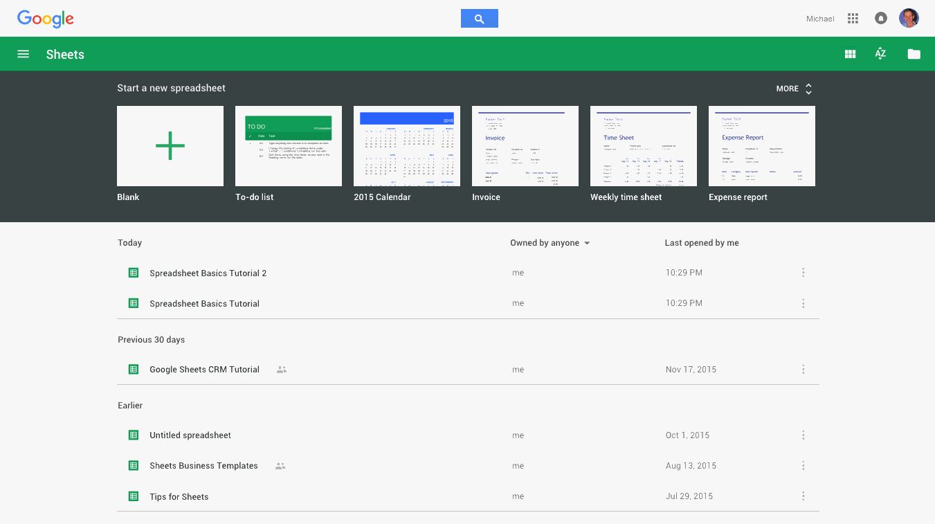
There are 3 ways to create a new spreadsheet in Google Sheets:

1. Click the red "NEW" button on your your Google Drive dashboard and select "Google Sheets"
2. Open the menu from within a spreadsheet and select "File > New Spreadsheet"
3. Click "Blank" or select a template on the Google Sheets homepage

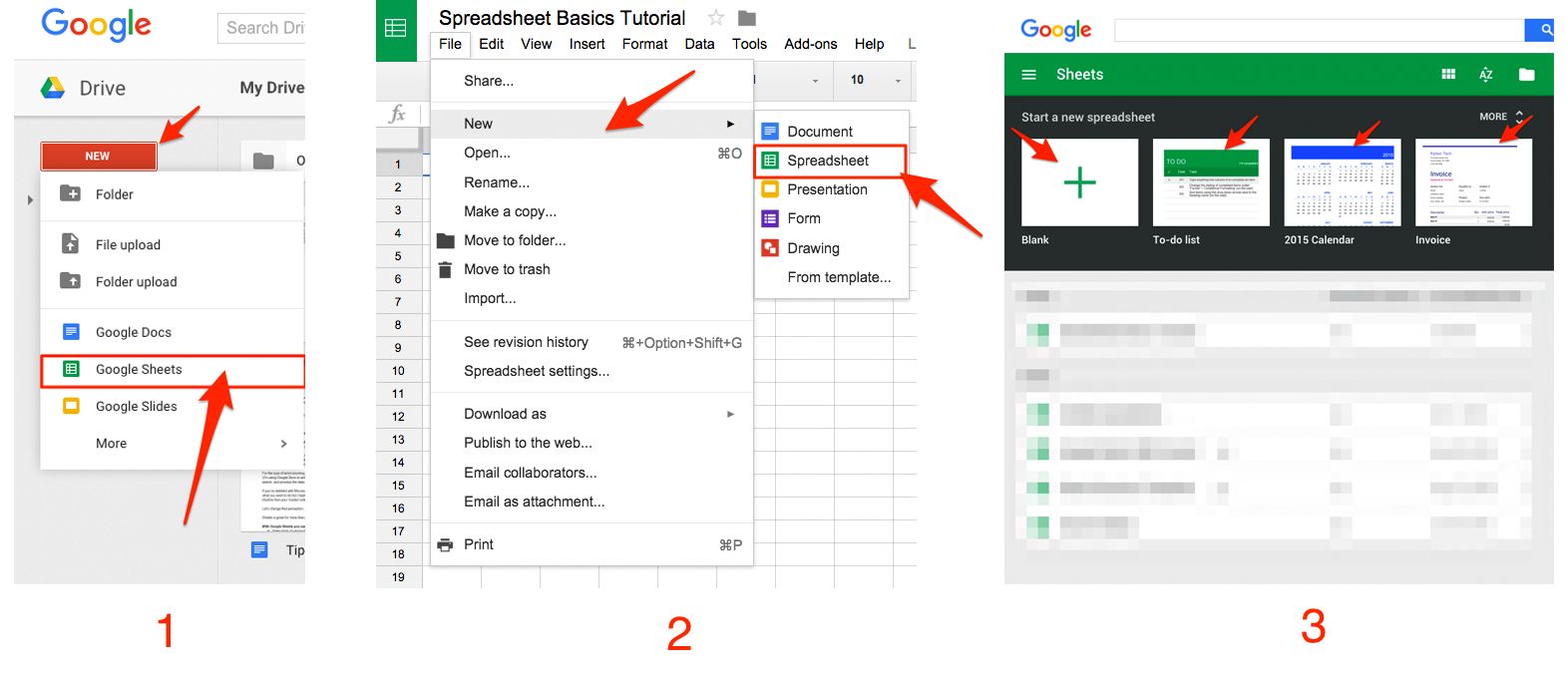
This will create a new blank spreadsheet (or a pre-populated template if you choose one of those). For this tutorial, though, you should start with a blank spreadsheet.

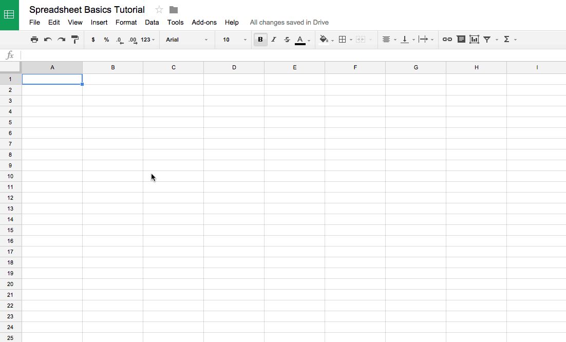
The Google Sheets interface should remind you of at least one other spreadsheet app you've seen before, with familiar text editing icons and tabs for extra sheets.

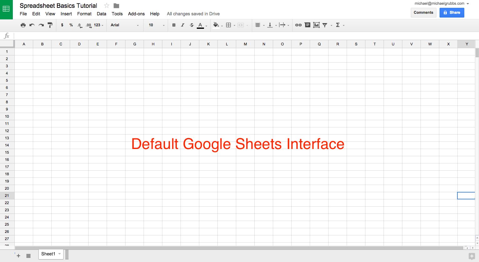
The only difference is that Google has reduced the clutter and number of displayed interface elements. So your first task should be obvious: Add some data!

Adding Data to Your Spreadsheet

Look around the white-and-grey grid that occupies most of your screen, and the first thing you'll notice is a blue outline around the selected cell or cells.

As soon as you open a new spreadsheet, if you just start typing you'll see that your data starts populating the selected cell immediately—usually the top left cell. There's no need to double click cells when you add information, and not much need to use your mouse.

An individual square in a spreadsheet is called a cell; they're organized into rows and columns with number and letter IDs, respectively. Each cell should contain one value, word, or piece of data.

Feel free to select any cell you'd like, then go ahead and type something in. When you're done entering data into a cell, you can do one of 4 things:

1. Press ENTER to save the data and move to the beginning of the next row
2. Press TAB to save the data and move to the right in the same row
3. Use the ARROW KEYS on your keyboard (up, down, left, and right) to move 1 cell in that direction
4. Click any cell to jump directly to that cell

If you don't want to type in everything manually, you can also add data to your Sheet en masse via a few different methods:

1. Copy and paste a list of text or numbers into your spreadsheet
2. Copy and paste an HTML table from a website
3. Import an existing spreadsheet in csv, xls, xlsx and other formats
4. Copy any value in a cell across a range of cells via a click and drag

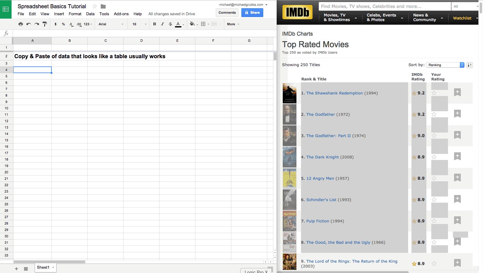
Copy & Paste is pretty self-explanatory, but there are times when you'll try to copy a "spreadsheet-y" set of data from a website or PDF, and it will just paste into one cell or format everything with the original styling. Try looking for data that's actually in an HTML table (like movie data from IMDB, for example) to avoid getting funky pasted data in your spreadsheet.

Note: Make sure you only click once on a cell before pasting data, so Google Sheets will turn it into a list with each item in its own cell. If you double-click on a cell, Google Sheets will paste all the data into one cell which is likely not what you want.

If you do end up with oddly formatted data, don't worry: we'll fix that in the next section!

Importing a file is simple as well. You can either import directly into the current spreadsheet, create a new spreadsheet, or replace a sheet (i.e. an individual tab) with the imported data.

The most common files you'll import are CSV (comma separated values) or XLS and XLSX (files from Microsoft Excel). To import a file from outside of your Google Drive, go to the FILE > IMPORT > UPLOAD menu.

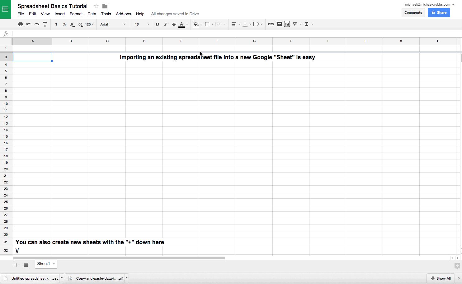
I prefer to import the data into a new sheet every time to keep my old data and new imported data separate. Alternatively, if you have a Google Sheet (or a CSV, XLS, or other spreadsheet file) saved in your Google Drive account, you can import that directly into your spreadsheet using the same process—just search your Drive from the import window.

Dragging to copy a cell value needs a bit of explanation, because you'll use this one a lot once you've set up formulas in your spreadsheets.

By dragging the small blue dot (pictured below) in the bottom-right corner of a highlighted cell across or down a range of cells, you can perform a number of different functions.

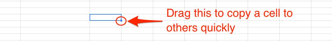
There are a number of ways you could use this feature:

1. Copying a cell's data to a number of neighboring cells (including formatting)
2. Copying a cell's "Formula" to neighboring cells (this is an advanced feature, and we'll cover it in detail later)
3. Creating an ordered list of text data

Here's an example of how to creating an ordered list might work: Try adding the text Contestant 1 to Cell A1, then clicking and dragging the little blue dot in the bottom-right corner of the highlighted cell either down or across any number of neighboring cells.

If there was no number after Contestant, this dragging action would simply copy "Contestant" to any cells you drag over. But because the number is there, Sheets knows to increment the next cell +1.

Let's assume that you have either copied, pasted, imported, or typed-in a good chunk of data, and that your spreadsheet is looking pretty healthy.

Now, How can we use this data?

---

2. Format Data for Easy Viewing

Whether you're tracking expenses, recording students' grades, or keeping track of customers in a homebrew CRM (as we'll build in chapter 3), you'll want to manipulate and format your data.

The basic formatting options in Google Sheets are available above your first cell. They're labeled in the image below, but for quick reference while you're working on a sheet, just hover over an icon to see its description and shortcut key.

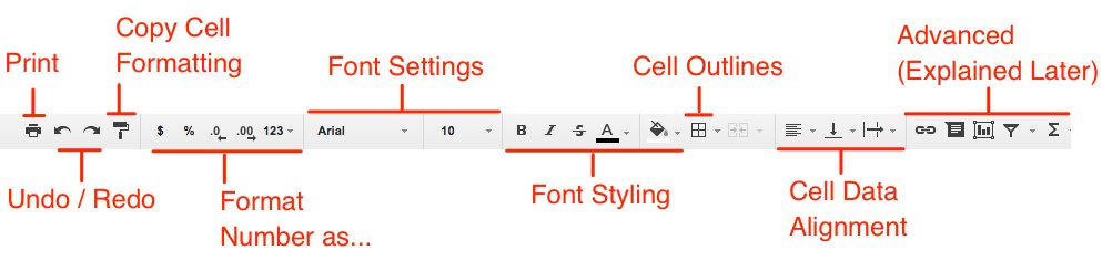
Print, Undo / Redo, and the Font Settings / Styling function similarly to what you'd expect from your favorite word processor. The shortcut keys are the same as well, so just treat it like you're editing any other document!

As for everything else, the best way to show you how everything works is to dive right into an example.

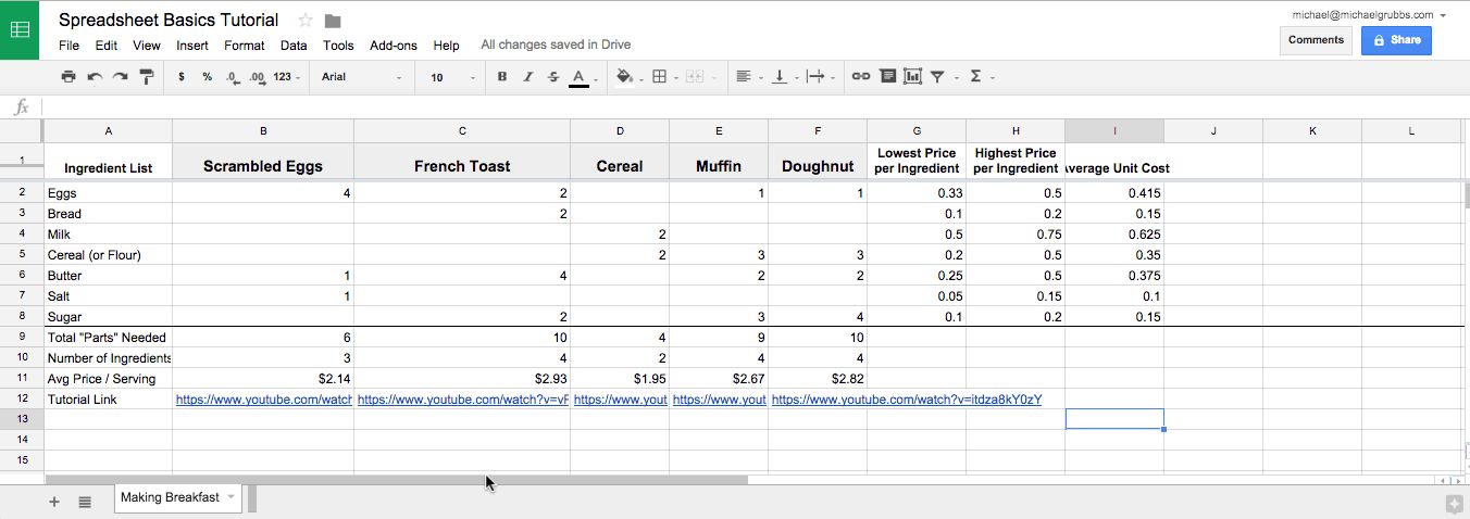
I'm going to create a quick list of potential breakfast options for tomorrow morning, along with their ingredients, counts, prices, and links to YouTube videos for how to make them (who knew you could make a 3-minute video about scrambled eggs?).

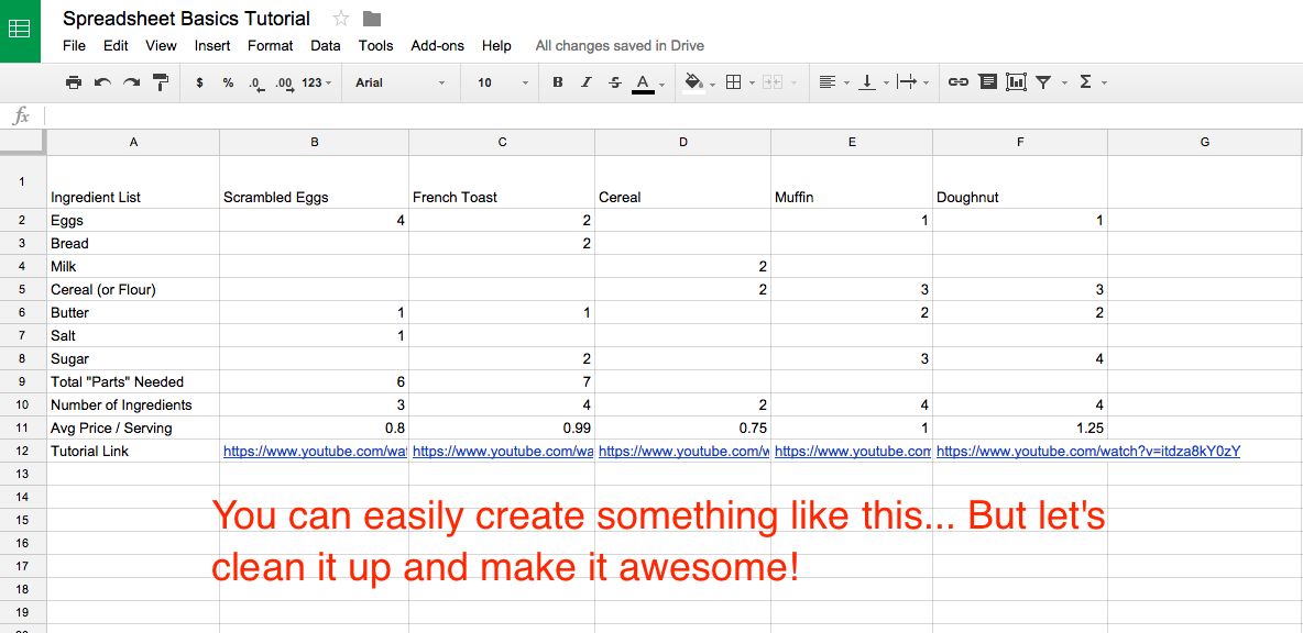
It's functional, enough that you could use this very easily to keep track of information. In fact, a vast majority of my own spreadsheets look like this—Google Sheets makes it so simple to capture information, share it, and return to it later for reference that it acts as my highly-structured note-taking tool.

But let's assume that you have to deal with dozens of spreadsheets per day (or worse, that you have to share spreadsheets back-and-forth) and this is what someone sends you. It's really boring, and if it was a large data set it would be painful to skim through.

For the simple example above a lack of significant formatting is "okay." It does the basics, storing my information and allowing me to save it. But it's not something I would want to come back to each day.

Since I eat breakfast every morning, let's take some time to make this spreadsheet more user-friendly with some formatting!

First we'll "Freeze" the first row in place. That means if we scroll down the spreadsheet, the first row will still be visible, no matter how much data lies below it. This allows you to have a long list and helps to keep tabs on what you're actually looking at.

There are two ways to freeze rows:

1. Click VIEW > FREEZE > 1 ROW in the navigation bar to lock the first row in place
2. Hover the dark grey bar in the top left of the spreadsheet (until it becomes a hand) and drag between rows 1 and 2

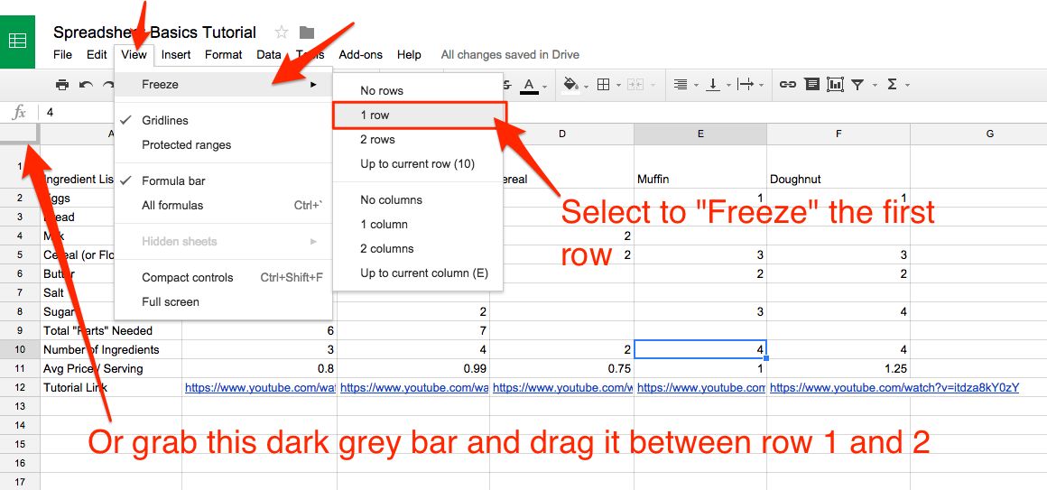
Freezing my header row is the first thing I do in every sheet I make.

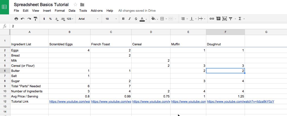
Now, let's make the header text pop with some simple text formatting (remember, the text formatting tools are in the toolbar, just above your first row):

1. Drag to select the cells you want to format
2. Bold the text
3. Increase font size to 12pt
4. Center-align the whole row
5. Give give your cells a grey fill

The next thing I'll do to clean this up a bit is format my "Average Price / Serving" to be a dollar value. Here's how things look at first:

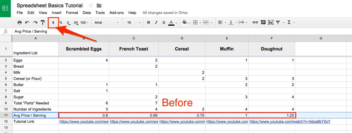
Now, let's clean that up with the "Format as $" button for the specific values (or entire row) highlighted.

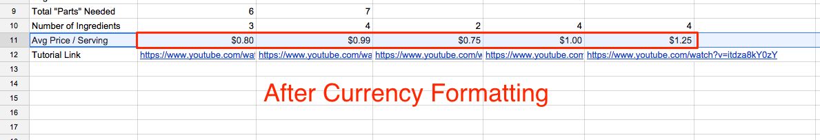
You'll see that your selected cells are now displayed as a dollar amount, rather than a regular number.

Note: if you perform this operation with the whole row / column highlighted, future values will take the formatting as well!

Now that you've got the hang of inserting and formatting your data, it's about time we start actually calculating some sums, averages, and more from your data!

---

3. Add, Average, and Filter Data with Formulas

Google Sheets, like most spreadsheet apps, has a bunch of built-in formulas for accomplishing a number of statistical and data manipulation tasks. You can also combine formulas to create more powerful calculations and string tasks together. And if you're already accustomed to crunching numbers in Excel, the exact same formulas work in Google Sheets most of the time.

For this tutorial, we'll focus on the five most common formulas, which are shown in the formula drop down menu from the top navigation.

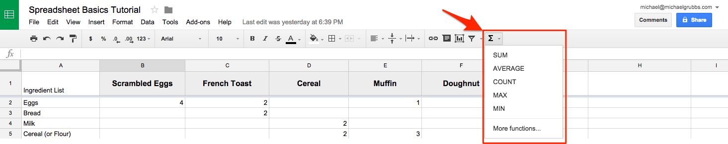
You can click a formula to add it to a cell, or you can start typing any formula with a = sign in a cell followed by the formula's name. Sheets will auto-fill or suggest formulas based on what you type, so you don't need to remember every formula.

The most basic formulas in Sheets include:

• SUM: adds up a range cells (e.g. 1+2+3+4+5 = sum of 15)
• AVERAGE: finds the average of a range of cells (e.g. 1,2,3,4,5 = average of 3)
• COUNT: counts the values in a range of cells (ex: 1,blank,3,4,5 = 4 total cells with values)
• MAX: finds the highest value in a range of cells (ex: 1,2,3,4,5 = 5 is the highest)
• MIN: finds the lowest value in a range of cells (ex: 1,2,3,4,5 = 1 is the lowest)
• Basic Arithmetic: You can also perform functions like addition, subtraction, and multiplication directly in a cell without calling a formula

We'll explore these formulas by improving our breakfast spreadsheet.

Using the SUM Formula

Let's start with adding up the total number of ingredients required for each recipe. I'll use the SUM formula to add each value in the recipes and get a total amount.

There are three ways to use the basic formulas accessible via the top navigation:

1. Select a range then click the formula (this will put the result either below or to the side of the range).
2. Select the result cell (i.e. the cell where you want the result to appear), then click on the formula you want to use from the toolbar. Finally, select the range of cells to perform your operation on.
3. Type the formula into the result cell (don't forget the = sign) then either manually type a range or select the range

I'll demonstrate all three methods in the gif below. First, I'll sum my ingredients by selecting a range, and clicking SUM from the formula menu. Second, I'll select a result cell and highlight the range of cells to be summed together. Finally, I will demonstrate typing a formula and range manually.

Note: In order to select a range of cells, click the first cell and hold SHIFT then click the last cell in the range. So if you want A1 through A10, click A1 then hold SHIFT and click A10.

When you've finished selecting the cells that you want to add together, press ENTER.

In my example, you see a grey help section pop up when I start typing the formula. When you create a formula for the first time, you'll instead notice a blue highlight and a question mark next to the cell.

You can click the question mark to toggle help context for formulas on or off. These tips will tell you what type of information can be used in each formula, and will make your formula creation (especially when you start combining formulas) much easier.

Now that we have a formula set up to SUM all of the ingredients together, let's make sure that it applies to all of the cells in that row. I'll select my formula cell and drag the blue dot across the other cells to copy the formula to those cells.

You'll notice that when you copy the formula to a neighboring cell, it shifts the range that the new formula is referencing. For instance, in the "Scrambled Eggs" column it was SUM(B2:B8) but in "French Toast" it's SUM(C2:C8).

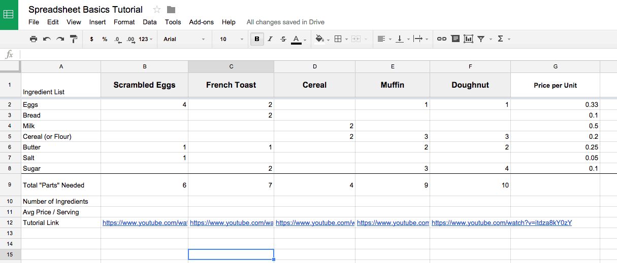
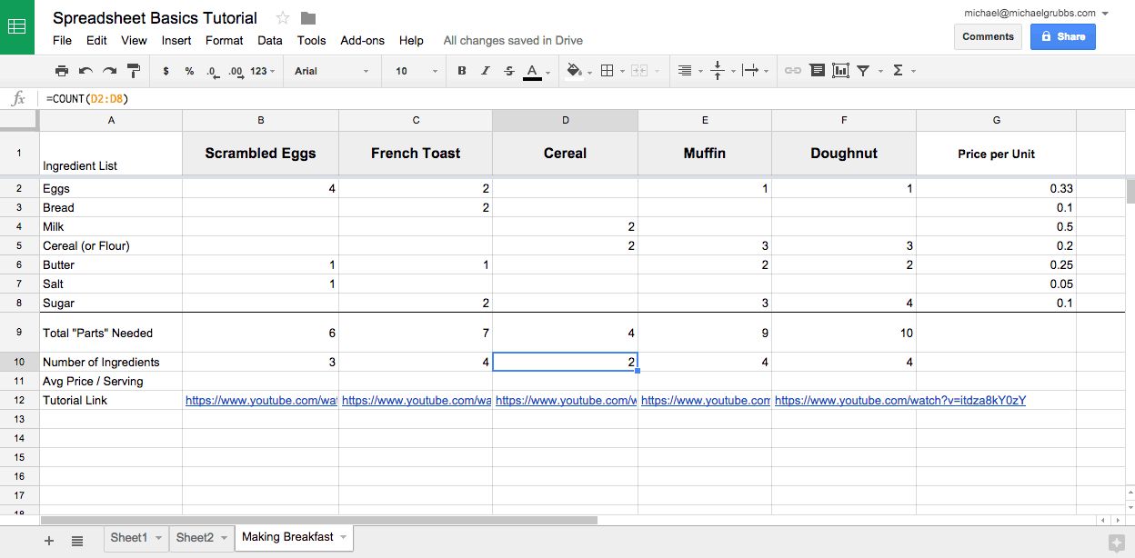
Using the COUNT formula

Now that we know how many parts are needed for each recipe, I'd like to know how complicated it is to make. I've simplified this by assuming that fewer ingredients means that the recipe is less complicated.

In order to count the number of ingredients in each recipe, I'll use the COUNT formula.

The count formula essentially checks to see if the cells in a range are empty or not, and returns the total that are filled.

This formula will be set up in my spreadsheet the same way as my SUM row.

Here's a trick we didn't cover in the previous section, though: highlight the cell range that you're trying to count and checking in the bottom right corner of your spreadsheet. If you've highlighted a pure list of numbers, Sheets will automatically SUM them for you and display the result. If you've highlighted a mixed range of numbers and text, it will COUNT the values.

You also have the option to perform any of the five number-based operations on a range of numbers by clicking the SUM button in the bottom right and selecting the new default formula from the pop-out menu. From then on, anytime you highlight a range it will perform the last-selected formula.

So according to my spreadsheet, "Cereal" is the least complicated breakfast, but I'm still not convinced that an easy breakfast is worth it.

What if it costs too much? What if the extra effort of cooking another meal saves me money?

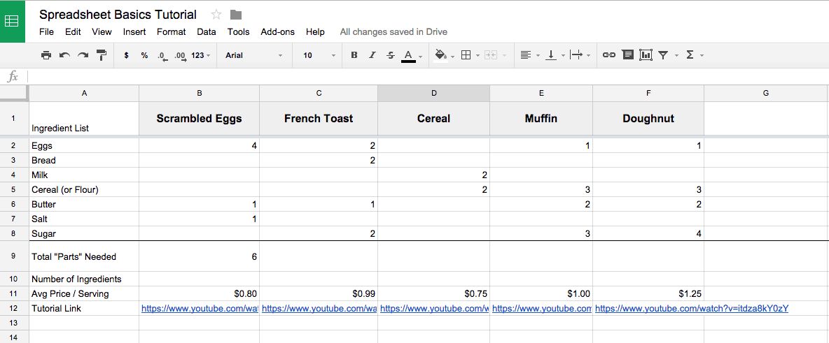
Let's refine our decision by figuring out the average cost per serving of the breakfast choices by using the AVERAGE formula.

Using the AVERAGE formula

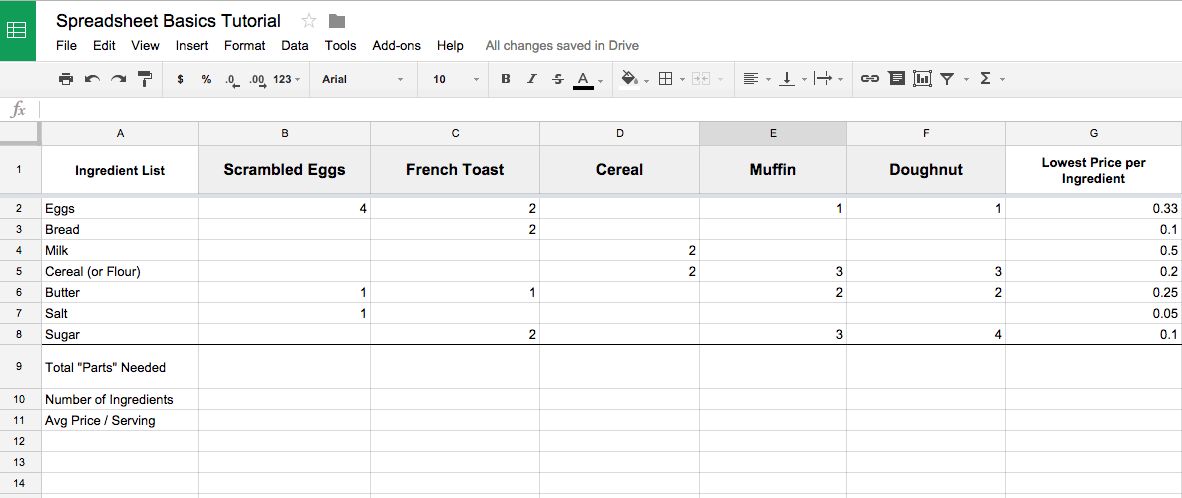
I've added some faux minimum and maximum prices per unit on my ingredients list to the right of my breakfast options. We'll want to get an average price for each ingredient using the low and high rates, then multiply the resulting average price of the ingredient by its respective unit count in each recipe.

I'll start by highlighting the range of values (in this case it's two side-by-side rather than a vertical range) and selecting the AVERAGE formula from the toolbar.

This will drop the result into the column to the right of the maximum price column. Next, I drag the formula down to apply it to the other min and max price combinations.

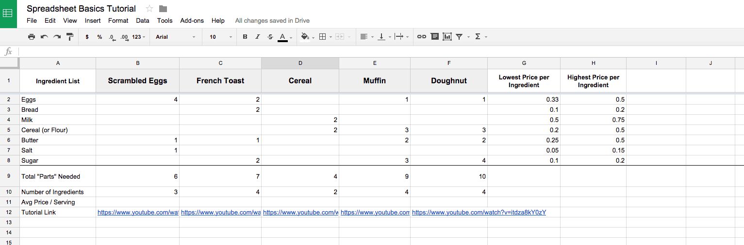
I'll label my column "Average Unit Cost" so we know what we're looking at. Then, let's move on to calculating the cost of the breakfast using simple arithmetic.

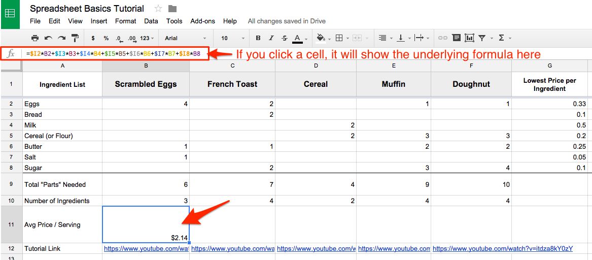
Using Simple Arithmetic Formulas

We need to calculate the total cost of the breakfast by multiplying the average price of each ingredient by its unit count in the recipe. To accomplish this, manually type a formula into the "Avg Price" row.

Our basic arithmetic formula would look like this for the "Scrambled Eggs" column:

=$I2*B2+$I3*B3+$I4*B4+$I5*B5+$I6*B6+$I7*B7+$I8*B8

The $ symbol before column I (the average prices) tells Sheets that no matter where we put the formula in our spreadsheet, we always want to reference the I column.That way, if we copy the formula to the other recipes, it will always use the average unit cost column rather than shifting the reference to the next column over when you drag to copy (like it did in the SUM and COUNT examples).

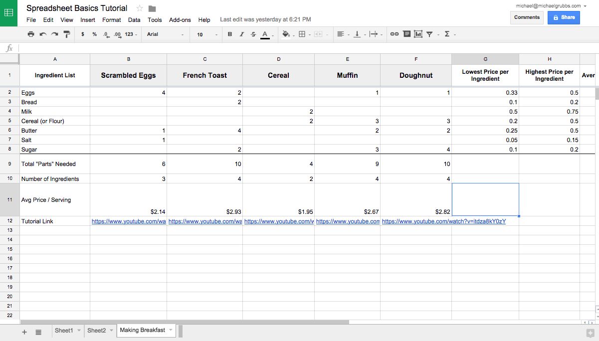
If you don't want to type those values in manually, there are cleaner ways to perform this type of formula: You could accomplish the same price calculation by using this advanced formula:

=SUM(ARRAYFORMULA(B2:B8*$I2:$I8))

There are many formulas in Sheets that take care of complex tasks for you, many of which we'll dig into in the next chapters.

Now that we have some working data and calculations, perhaps my coworkers (who are likely planning to eat breakfast tomorrow) might benefit from this sheet.

Let's prepare to share our spreadsheet, and invite some collaborators to view, edit, and use our data.

---

4. Share, Protect, and Move Your Data

What makes Sheets so powerful is how "in sync" you'll feel with your coworkers. Jointly editing a spreadsheet is one of the critical functions of Sheets, and Google has made it a seamless experience.

Here's how it works:

1. Click either FILE > SHARE or use the blue "Share" button in the top right
2. Click "advanced", then enter emails of who can view or edit your spreadsheet
3. Select any other privacy options and hit done

When you open the "advanced" sharing panel, you'll see a number of options.

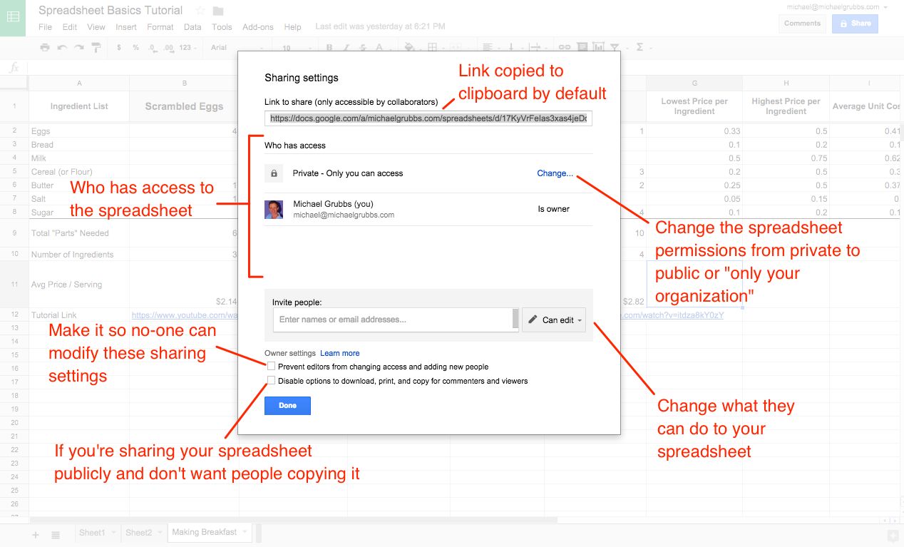
The default functionality when you click the "Share" Button is to copy a link to the spreadsheet to your clipboard.

When you share this link with someone via a messenger or email, if they click the link it will bring them to the spreadsheet. However, unless you've invited them via email (in the email field) and selected "Can Edit", they will still need to request permission to make changes.

If you'd like to give anyone within your organization or company editor-level access, click the "change…" button in the "Who has Access" section and select "On - (Your Organization Name)**". (Note: this option will only appear if you're using Google Apps for Work.)

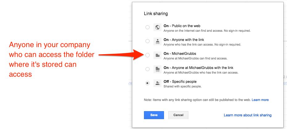
Someone is "In your organization" when they have an email address and Google account for your company. In this case, I've named by "company" MichaelGrubbs, so everyone in my organization has an @michaelgrubbs.com email address and anyone signed in to one of those accounts can access the spreadsheet.

You can learn more about sharing and permissions here—you'll want to make sure you are using the right permissions for the audience you're sharing with.

Sharing Spreadsheets with Your Devices and Apps

Even though Google Sheets and Drive are built for sharing between users, you'll notice that many times your spreadsheets are created as internal documents, and sharing is secondary to actually getting work done.

You can streamline your spreadsheet workflows and real-time data-sharing by taking advantage of these helpful add-ons:

1. The Google Docs mobile apps. You can use the Google Sheets mobile app to view and edit your spreadsheets, share links on the go, and add users. It's a solid companion to—but not a replacement for—the web app.
2. Google Drive sync to your desktop. Google Drive allows you to easily upload files from your local desktop environment to your online Drive. This makes them accessible to your collaborators and also allows you to quickly import them into spreadsheets and other documents.
3. A Third-Party tool like Zapier. You can use Zapier to automatically add data to your spreadsheets, send files to your Google Drive account, alert you of change to your Sheets… you name it

Let's continue working on our spreadsheet example to demonstrate using Zapier, an app integration tool, to make Google Sheets even more powerful.

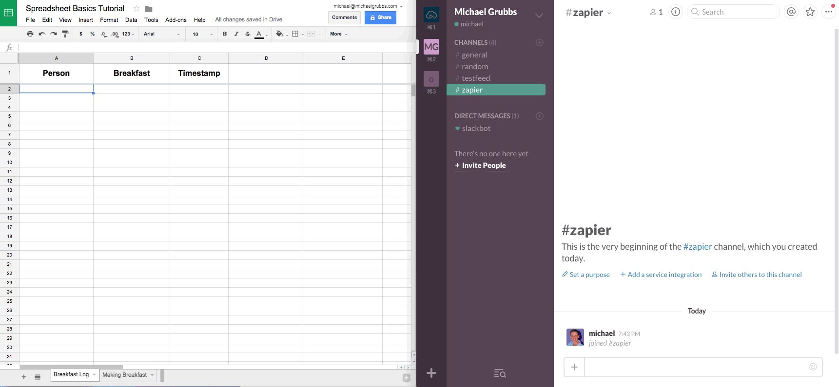
Rather than hitting the "Share" button on my spreadsheet to send it to my colleagues, I'd like to send a Slack message alerting them that I've created this new spreadsheet.

You can automatically send a message to a Slack channel with Zapier's Google Sheets Trigger and Slack Action.

I've set my Zap up to look for new Spreadsheets in my Google Drive then post the file name and a link to the spreadsheet in a Slack Channel.

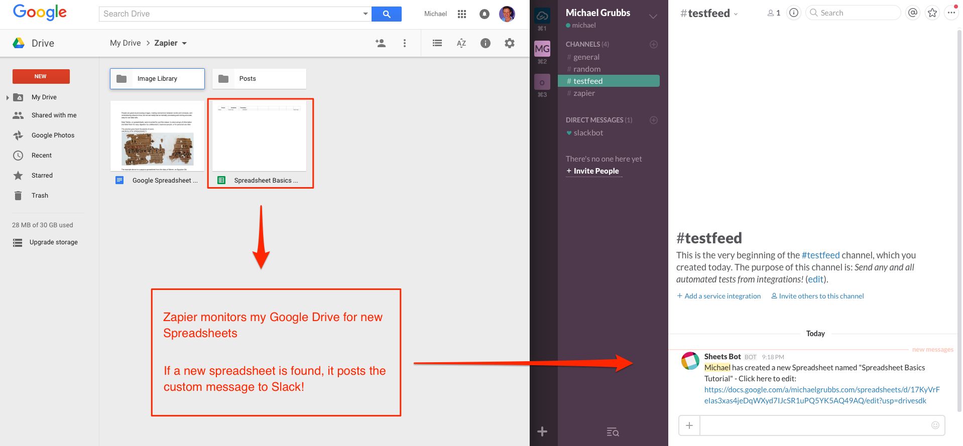
This is great for updating your team when you create new documents that you'd like to quickly loop everyone in on.

You can set up filters and conditions to decide when to post, and you have complete control over what information you'd like to include in your message. You can also trigger messages based on different actions in Google Sheets—like when someone a new row or changes the data in a cell. Check out the Zapier's Google Sheets page for more information on supported data and triggers.

Now let's switch the direction of the data-flow and consider how our colleagues would interact with our Spreadsheet.

I'd like to allow myself and my team to interact with my spreadsheet and keep track of what they had for breakfast in a breakfast log. Without an automation tool like Zapier, tasks like this quickly become the reason that people fail to collaborate successfully using spreadsheets.

Think about it, if this were a normal spreadsheet without any automation, you'd be asking someone to:

1. Break out of their current activity
2. Track down the spreadsheet
3. Fill in a few pieces of potentially inconsequential data
4. Save and re-share this file (if it's not already an online and synced document)
5. Repeat for any number of tasks / documents

This is where automating tasks becomes so vital.

Let's set up our spreadsheet so that it has a clean sheet to receive some automated data. I'll create a new worksheet using the + button in the bottom left.

Now, I'll use Zapier again and make Slack the triggering action with Google Sheets on the receiving end of the automation (the "Action" side of the Zap).

I've set up my Zap to instantly take a Slack message posted into a dedicated channel and create a new row in the breakfast log along with the time and user who posted it.

Check it out in real-time:

And this can work for hundreds of other applications that you can use as Triggers or Actions with Zapier. You can send information to your spreadsheet via email, monitor your social channels, set it on a schedule; there are dozens of different ways to accomplish any given task with the apps you're already using.

Downloading Your Data

If you need to send your files to external collaborators, upload a file into another system, or just like having backups for posterity, then turn towards one of Google Sheets' many data export options.

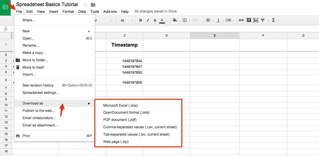
The most common exports will be either .xls (Excel document) or .csv (comma-separated values). If you're not sure which format to use, a .csv is usually the best bet.

Use Your Spreadsheet in Offline Mode

If you love what you've seen so far but were worried that you wouldn't be able to use Sheets without a connection, then fear not. Google Sheets has an "Offline Mode" that will automatically sync your changes to the document when you reconnect to the internet.

This is useful for any situation where you'd need to treat Google Sheets like a desktop application—on a flight or a road trip, for example.

Here's what you'll need:

1. Google Chrome
2. Google Drive Chrome Web App
3. Google Drive Sync

Instructions for setting up your offline sync are really straight-forward, but the bulk of the process is just downloading and using the three core components above.

Actually turning it on looks like this (get ready to be amazed):

And just like that, you can use Google Sheets even when you're offline—no WiFi necessary.

For more tips on using Google Sheets offline, jump to the end of chapter 6.

---

That's All For Now

Here's what you've just learned how to do if you followed along for the whole chapter (you can hit each link to back-track):

1. Create a new spreadsheet
2. Add data to your sheet and format it
3. Set up formulas to calculate tabular data
4. Share your spreadsheet with collaborators or the world
5. Connect and automate your Sheets with Third-party apps
6. Download your Spreadsheet data
7. Use Google Sheets offline from anywhere

---

Google Sheets is a powerful tool—it's everything you'd expect from a spreadsheet, with the extra perks of an online app. While the example spreadsheet that we created may have been a bit silly, the practical applications of using Sheets for your workflows (both business and personal) are limitless.

Whether you need to make a budget, outline your next proposal, gather data for a research project, or log info from any other app that connects with Zapier, a Google Sheets spreadsheet can bring your data to life. And with everything stored in Google Drive, you'll never worry about losing your files again—even if your computer dies.

---

Now that you know how to make a spreadsheet, it's time to fill your spreadsheet with data. The best way to do that in an online spreadsheet is with a form—and in chapter 2, we'll look at the free Google Forms tool that can help you gather data and save it directly to your spreadsheet.

Go to Chapter 2!

How To Use Google Sheets On Iphone

Source: https://zapier.com/learn/google-sheets/google-sheets-tutorial/

Posted by: messerguill1987.blogspot.com

Share this post